

DN80 to DN2000: How to Select Correct Ductile Iron Pipe Diameter for Water Projects (2026 Guide)
DN80 to DN2000: How to Select Correct Ductile Iron Pipe Diameter for Water Projects
Selecting the correct ductile iron pipe diameter is one of the most critical decisions in water infrastructure design. The choice affects not only initial material and installation costs, but also long-term operating expenses, system reliability, and maintenance requirements. This comprehensive guide provides a systematic approach to pipe diameter selection from DN80 to DN2000, with practical calculations, real-world case studies, and lessons learned from actual projects.
")
The Cost of Getting Pipe Size Wrong
Before diving into calculation methods, it's important to understand the consequences of incorrect pipe sizing:
Undersizing Problems
High friction loss: Increased pumping energy costs (can be 2-3× design estimate)
Low pressure at endpoints: Customer complaints, fire flow inadequacy
Excessive velocity: Pipe erosion, water hammer damage, noise
Limited expansion capacity: Cannot accommodate future growth without expensive replacement
Frequent pump maintenance: Pumps operating outside optimal efficiency curve
Oversizing Problems
Excessive material cost: Each diameter increase adds 25-35% to pipe cost
Larger trench excavation: Wider trenches mean more earthwork and restoration cost
More expensive fittings: Elbows, tees, valves cost significantly more for larger sizes
Water age issues: Low flow velocity leads to water stagnation and quality degradation
Sediment accumulation: Velocity below 0.3 m/s allows particles to settle
Systematic Pipe Sizing Method: 4-Step Approach
Follow this proven methodology to select optimal pipe diameter:
Step 1: Calculate Design Flow Rate
The foundation of pipe sizing is accurate flow rate estimation. Use this systematic approach:
Method A: Population-Based Calculation (Municipal Systems)
Qavg = average daily flow (m³/day)
P = population served (persons)
q = per capita consumption (liters/person/day)
Typical per capita consumption values:
| Region/Type | Per Capita Consumption (L/person/day) | Notes |
|---|---|---|
| Rural areas (developing) | 80-120 | Basic water supply |
| Urban areas (developing) | 120-200 | Standard municipal |
| Developed countries | 200-350 | High consumption |
| Industrial zones | 300-500 | Includes industrial use |
| Commercial districts | 150-250 | Offices, retail |
Example Calculation:
A town with 50,000 population, per capita consumption 180 L/person/day:
Peak Flow Calculation
Design for peak flow, not average flow:
Qmax = maximum daily flow (m³/day)
PF = peak factor (typically 1.5-2.5)
Peak factor selection:
Small systems (<10,000 population): PF = 2.5-3.0
Medium systems (10,000-100,000): PF = 2.0-2.5
Large systems (>100,000): PF = 1.5-2.0
Continuing the example with PF = 2.2:
Method B: Area-Based Calculation (New Developments)
For new residential or industrial developments where population is unknown:
A = service area (hectares)
D = population density (persons/hectare)
q = per capita consumption (L/person/day)
PF = peak factor
Typical population densities:
Low-density residential: 30-50 persons/hectare
Medium-density residential: 80-150 persons/hectare
High-density residential: 200-400 persons/hectare
Industrial zones: 10-30 persons/hectare (employment-based)
Method C: Fixture Unit Method (Building Connections)
For DN80-DN150 building service connections, use fixture unit method per local plumbing code.
Step 2: Determine Allowable Velocity
Water velocity significantly impacts system performance and pipe longevity:
Velocity Guidelines by Application
| Application | Minimum Velocity | Optimal Velocity | Maximum Velocity |
|---|---|---|---|
| Water distribution (municipal) | 0.5 m/s | 0.8-1.2 m/s | 1.5 m/s |
| Transmission mains | 0.8 m/s | 1.2-1.8 m/s | 2.0 m/s |
| Pump discharge | 1.0 m/s | 1.5-2.0 m/s | 2.5 m/s |
| Gravity flow | 0.3 m/s | 0.6-1.0 m/s | 1.2 m/s |
| Fire protection | 1.0 m/s | 2.0-2.5 m/s | 3.0 m/s (emergency) |
Velocity Constraints Explained
Minimum Velocity (0.5-0.8 m/s):
Prevents sediment deposition
Maintains chlorine residual throughout system
Avoids water age and quality degradation
Ensures self-cleansing action
Maximum Velocity (1.5-2.0 m/s for most applications):
Limits friction head loss and pumping costs
Reduces water hammer risk during valve closure
Prevents pipe erosion and cavitation damage
Minimizes noise in residential areas
Diameter from Flow and Velocity
D = internal diameter (m)
Q = flow rate (m³/s)
v = velocity (m/s)
π = 3.14159
Example: For Q = 229 L/s (0.229 m³/s) and v = 1.2 m/s:
Nearest standard size: DN500 (actual ID ≈ 514mm for K9)
Step 3: Check Pressure Loss
Verify that selected diameter provides acceptable pressure loss over pipeline length.
Hazen-Williams Equation (Most Common for Water)
hf = friction head loss (meters)
L = pipe length (meters)
Q = flow rate (m³/s)
C = roughness coefficient
D = internal diameter (meters)
Hazen-Williams C values for ductile iron pipe:
New pipe with cement lining: C = 140-150
10-year-old pipe: C = 130-140
20-year-old pipe: C = 120-130
Design (conservative): C = 130
Example: DN500 K9 pipe, L = 15,000m, Q = 0.229 m³/s, C = 130, D = 0.514m
= 10.67 × 15000 × 0.0677 / (8463 × 0.0443)
= 10,840 / 375 = 28.9 meters
Pressure loss = 28.9m / 15km = 1.93 m/km (acceptable for transmission main)
Acceptable Pressure Loss Guidelines
| Pipeline Type | Max Loss (m/km) | Optimal Range (m/km) |
|---|---|---|
| Distribution mains | 5.0 | 2.0-4.0 |
| Transmission mains | 3.0 | 1.0-2.5 |
| Pump discharge | 8.0 | 3.0-6.0 |
| Gravity systems | 2.0 | 0.5-1.5 |
Darcy-Weisbach Equation (More Accurate)
For critical projects or when higher accuracy is needed:
f = Darcy friction factor (from Moody chart or Colebrook equation)
L = pipe length (m)
D = internal diameter (m)
v = velocity (m/s)
g = gravitational acceleration (9.81 m/s²)
Step 4: Evaluate Lifecycle Cost
Optimal pipe diameter minimizes total lifecycle cost, not just initial investment.
Cost Components Over 50-Year Life
| Cost Component | Typical % of LCC | Varies With Diameter? |
|---|---|---|
| Pipe material | 15-20% | Yes (increases with size) |
| Installation (trench, laying) | 25-30% | Yes (increases with size) |
| Fittings and valves | 10-15% | Yes (increases with size) |
| Pumping energy (50 years) | 30-40% | Yes (decreases with size) |
| Maintenance | 5-10% | Minimal variation |
Lifecycle Cost Analysis Method
Compare 2-3 candidate diameters:
Calculate initial cost: Pipe + fittings + installation for each diameter
Calculate annual pumping cost: Based on friction loss and electricity rate
Calculate NPV of pumping cost: Over 50 years at appropriate discount rate
Add initial + NPV: Select diameter with lowest total
LCC = lifecycle cost
Cinitial = initial capital cost
Cpump = annual pumping cost
r = discount rate (typically 6-8%)
n = year (1 to 50)
Case Study: 20km Transmission Main
Project: Raw water transmission, Q = 350 L/s, L = 20km
Option A: DN600 K9
Initial cost: $2.8 million
Friction loss: 2.8 m/km → Total head: 56m
Annual pumping cost: $142,000
NPV (50yr, 7%): $1.95 million
Total LCC: $4.75 million
Option B: DN700 K9
Initial cost: $3.6 million (+28%)
Friction loss: 1.4 m/km → Total head: 28m
Annual pumping cost: $71,000
NPV (50yr, 7%): $0.98 million
Total LCC: $4.58 million
Option C: DN800 K9
Initial cost: $4.5 million (+61%)
Friction loss: 0.7 m/km → Total head: 14m
Annual pumping cost: $35,000
NPV (50yr, 7%): $0.48 million
Total LCC: $4.98 million
Conclusion: DN700 has lowest LCC despite 28% higher initial cost. Payback period: 11 years. DN800 is over-sized with diminishing returns.
Quick Selection Guide by Application
For preliminary planning, use these typical size ranges:
Municipal Water Distribution
| Service Population | Main Size | Branch Size | Service Connection |
|---|---|---|---|
| <5,000 | DN150-DN200 | DN100-DN150 | DN80-DN100 |
| 5,000-20,000 | DN200-DN300 | DN150-DN200 | DN80-DN100 |
| 20,000-50,000 | DN300-DN450 | DN200-DN300 | DN100-DN150 |
| 50,000-100,000 | DN450-DN600 | DN300-DN450 | DN100-DN150 |
| 100,000-500,000 | DN600-DN900 | DN400-DN600 | DN150-DN200 |
| >500,000 | DN900-DN1400 | DN600-DN900 | DN150-DN250 |
Industrial Water Supply
| Industry Type | Typical Flow | Recommended Size | Notes |
|---|---|---|---|
| Food & beverage | 50-200 L/s | DN200-DN350 | High quality requirements |
| Textile | 100-400 L/s | DN300-DN500 | Large cooling water demand |
| Chemical | 200-800 L/s | DN400-DN700 | Process + cooling water |
| Power plant | 500-2000 L/s | DN600-DN1200 | Cooling water dominant |
| Steel mill | 300-1500 L/s | DN500-DN1000 | High temperature considerations |
Irrigation Systems
| Irrigated Area | Flow Rate | Main Line Size | Sub-main Size |
|---|---|---|---|
| 100-500 hectares | 20-80 L/s | DN150-DN250 | DN100-DN150 |
| 500-2000 hectares | 80-300 L/s | DN300-DN500 | DN200-DN300 |
| 2000-5000 hectares | 300-800 L/s | DN500-DN800 | DN350-DN500 |
| >5000 hectares | 800-2000 L/s | DN800-DN1200 | DN500-DN700 |
Common Sizing Mistakes and How to Avoid Them
Mistake 1: Using Average Flow Instead of Peak Flow
Problem: Sizing pipe for average daily flow without considering peak factors.
Consequence: Inadequate capacity during peak hours, low pressure complaints, inability to meet fire flow requirements.
Solution: Always design for maximum daily flow (Qmax = Qavg × PF). For critical systems, also check hourly peak factor (typically 1.3-1.5× daily peak).
Mistake 2: Ignoring Future Expansion
Problem: Sizing only for current demand without considering growth.
Consequence: Pipe becomes undersized within 5-10 years, requiring expensive parallel line or replacement.
Solution: Design for 20-30 year horizon. Use population growth projections from urban planning department. For rapidly growing areas, consider installing larger diameter in phases or leaving room for parallel line.
Mistake 3: Not Checking Minimum Velocity
Problem: Focusing only on maximum flow, ignoring low-flow conditions.
Consequence: Water age, chlorine residual loss, sediment deposition, bacterial growth.
Solution: Verify velocity at minimum flow (typically 30-50% of average) is above 0.3-0.5 m/s. For systems with large flow variation, consider:
Installing smaller parallel line for low-flow periods
Using variable speed pumps to maintain velocity
Designing looped network for better flow distribution
Mistake 4: Overlooking Surge Pressure in Sizing
Problem: Sizing based on static pressure only, ignoring water hammer effects.
Consequence: Pipe bursts during pump trips or rapid valve closure, especially in long transmission lines.
Solution: Perform surge analysis for lines >2km. Consider:
Upsizing diameter to reduce velocity and surge magnitude
Installing surge tanks or air valves
Using soft starters or VFDs for pumps
Specifying slow-closing valves (≥10 seconds)
Mistake 5: Copying Designs Without Verification
Problem: Using pipe sizes from similar projects without recalculating for specific conditions.
Consequence: Sizes may be wrong due to different flow rates, lengths, elevations, or future plans.
Solution: Always perform fresh calculations for each project. Use previous designs as sanity check, not as basis for sizing.
How to Verify Pipe Supplier Capabilities for Your Project
Hydraulic performance calculations are only reliable when pipe dimensions match design specifications. Some foundries focus on small diameters (DN80-DN600), while others specialize in large pipes (DN800-DN2000). By integrating production capacity across qualified Chinese foundries, Tiegu delivers compliant and high-quality casting products to buyers worldwide while matching projects with suppliers whose production range aligns with specific requirements.
This avoids dimensional variations that can affect flow calculations and pressure ratings.
Submit your project specifications to receive supplier options with verified production records.
Hydraulic performance calculations are only reliable when pipe dimensions match design specifications. Some foundries focus on small diameters (DN80-DN600), while others specialize in large pipes (DN800-DN2000). Tiegu matches projects with suppliers whose production range aligns with project requirements.
This avoids dimensional variations that can affect flow calculations and pressure ratings. Supplier production records and dimensional inspection reports can be reviewed before order commitment.
Pipe Sizing Checklist
Conclusion
Selecting the correct ductile iron pipe diameter requires balancing hydraulic performance, initial cost, and long-term operating expenses. The 4-step methodology (flow calculation → velocity selection → pressure loss verification → lifecycle cost analysis) provides a systematic approach that avoids common pitfalls.
Key principles to remember:
Design for peak flow, not average - Include appropriate peak factors
Consider 20-30 year horizon - Account for population and demand growth
Optimize velocity - Target 0.8-1.5 m/s for most applications
Verify pressure loss - Use Hazen-Williams with conservative C factor
Evaluate lifecycle cost - Don't minimize initial cost at expense of operating cost
Check minimum flow - Ensure water quality at low-demand conditions
For complex projects or when internal expertise is limited, consider engaging hydraulic modeling consultants or requesting technical support from pipe suppliers. The cost of professional sizing assistance is minimal compared to the expense of correcting undersized or oversized pipe installations.
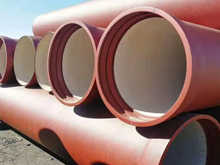
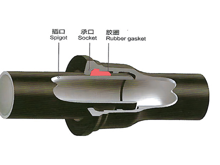 GT-type Joint Ductile Iron Pipe
 Sewage Pipe (Ductile Iron Sewage Pipe)
 Special Coating Pipe (Ductile Iron Pipe with Special Coatings)